This is part of my series on learning to build an End-to-End Analytics Platform project.
TLDR; After a suggestion from a friend (Waylon Payne LinkedIn) we start learning about time series database InfluxDB. We set up InfluxDB on the Raspberry Pi by creating a database. Work on getting Grafana installed and running. We write, troubleshoot, and learn a bunch logging data to InfluxDB. Finally we create a dashboard in Grafana to display on Sense HAT telemetry.
Begin the Influx 🌌
Last time we tackled writing out SenseHAT readings to a csv on the Pi. Now though, we level up by working on writing that data to a database more suited for streaming log data, in this case InfluxDB.
The InfluxDB documentation has a section for installing on a Raspberry Pi. Now while I was discussing this with my friend, he suggested before strolling down the path of flashing a new OS I should read this article Installing InfluxDB & Grafana on Raspberry Pi. Skipping step 0 is the plan in our case. Another post for references was Datalogger example using Sense Hat, InfluxDB and Grafana. Big thanks to Simon Hearne and Circuits.dk, their posts really helped guide my thinking even though I chose to do things a little differently. 😎
First up, some updates.
sudo apt update
sudo apt upgrade -y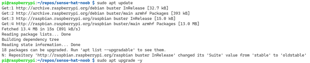
Updates ran pretty quickly. The next part is getting the InfluxDB packages.
wget -qO- https://repos.influxdata.com/influxdb.key | sudo apt-key add -
source /etc/os-release
echo "deb https://repos.influxdata.com/debian $(lsb_release -cs) stable" | sudo tee /etc/apt/sources.list.d/influxdb.list
A few things here to learn from the previous code snippets:
- apt – Is a command line package/software management tool on Debian (Debian Wiki) like search, installation, and removal.
- etc directory – Holds core configuration files. Found a nice Linux directory structure for beginners post.
- wget – Is a command line package/software for retrieving files using HTTP, HTTPS and FTP, the most widely-used Internet protocols (Debian Wiki).
- tee – Reads the standard input and writes it to both the standard output and one or more files (GeeksForGeeks).
- source – Reads and execute the content of a file (GeeksForGeeks).
Best I can understand at the moment is that we get and store a public key that allows us to authenticate/validate the InfluxDB package when we download it by echoing the latest InfluxData stable release package and adding the package deb record to the source.list directory in a new file which seem to allow apt-get to pick up future updates. That kicked off the install of InfluxDB. How do we know? The console says so..

It installs InfluxDB version 1.8.9 (not 2.0 which is the latest at the moment). Keep that in mind when working with documentation. Upgrading to 2.0 we can leave for the future. Onward!
sudo systemctl unmask influxdb.service
sudo systemctl start influxdb
sudo systemctl enable influxdb.service
More things to learn:
- sudo – Is not judo 🥋. It gives us Administrative capability to do things our standard accounts can’t like installing software.
- systemctl – Is a command line utility to interact with systemd. It covers way more, but what I mostly used it for was working with the services.
Found the command to check a service status with the –help switch for the systemctl command. These all feel reasonably familiar coming from working a little with PowerShell and the Windows terminal.
sudo systemctl --help
sudo systemctl status influxdb.service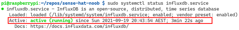
The service is up, active, and running. That means we should be able to connect to it. We can do that by logging into the Influx CLI from the terminal. Then creating a database. Creating a user. Finally, granting the user permissions.
influx

create '<yourdatabase>'

use '<yourdatabase>'

create user '<yourusername>' with password '<yourpassword>' with all privileges

grant all privileges on '<yourdatabase>' to '<yourusername>'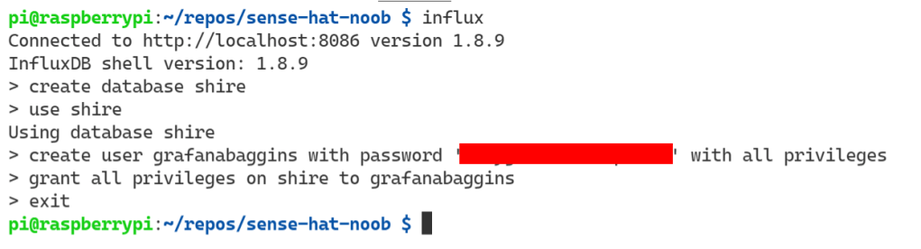
Ah familiar territory! A database! Now we have:
- A database service running.
- A database created.
- A user that has more than enough permissions to interact with the database.
Grafana
We want a way to visualise the telemetry that’s going to be written into the database. Grafana gives us the ability to create, explore and share all of your data through beautiful, flexible dashboards and we can run the service on the Pi. We’re taking the same approach as we did for InfluxDB to get Grafana up and going. Getting all the packages, installing them, running updates, and validating the services.
wget -q -O - https://packages.grafana.com/gpg.key | sudo apt-key add -
echo "deb https://packages.grafana.com/oss/deb stable main" | sudo tee /etc/apt/sources.list.d/grafana.list

sudo apt update && sudo apt install -y grafana

sudo systemctl unmask grafana-server.service
sudo systemctl start grafana-server
sudo systemctl enable grafana-server.service

sudo systemctl status grafana-server.service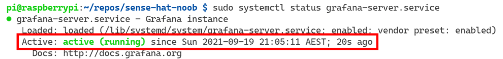
Once the service is up we should be able to connect to it on port 3000.
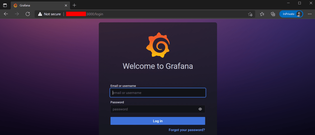
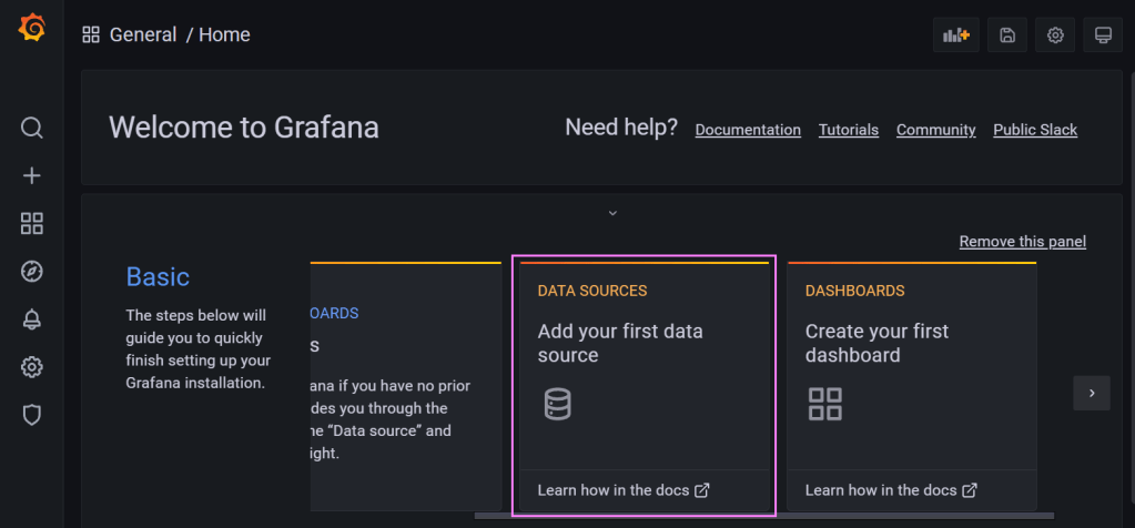
Yay! We’re connected. Let’s log in with the user name and password ‘admin‘ then reset the password. After the login process is done, we’ll land on the homepage for our Grafana instance running on the Pi. I’m actually excited about this 😄.
We need a way to connect Grafana to our InfluxDB database. On the Home page is a ‘Data Sources‘ tile which we can follow to add a data source.
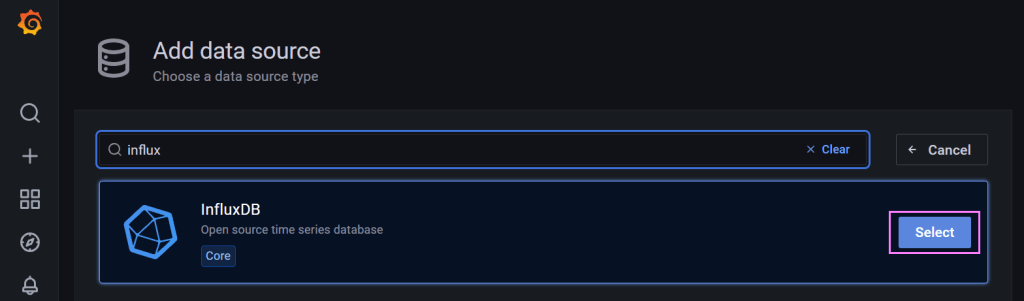
We can use the search box to lookup a connector for InfluxDB. Once we have that we just select it.
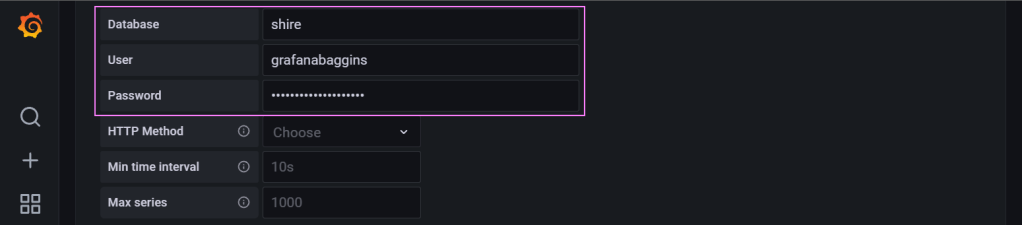
From there we configure the settings for the connector.
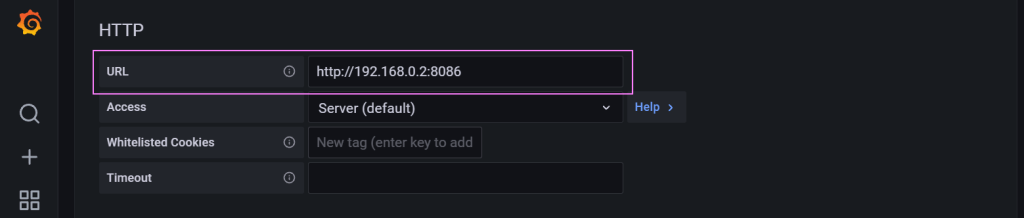
Credentials to make our way into the database.
Finally, we save and test the connector to make sure its all working.
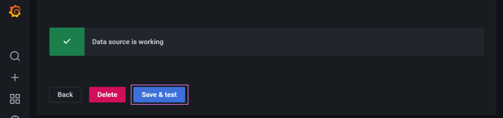
Good news. The scaffolding is in place. Now we need to get data into the database then configure some dashboards.
Bilbo Loggings 🪵
“If ever you are passing my way,” said Bilbo, “don’t wait to knock! Tea is at four; but any of you are welcome at any time!”
– Bilbo Baggins
Did someone say tea? Time for a spot of IoT! Now to get our IoT device capturing data. A quick swish of our telemetry logging code and we have a starting point. All we need to do is figure out how to log data to InfluxDB not the csv.
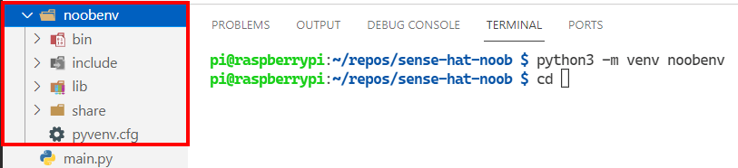
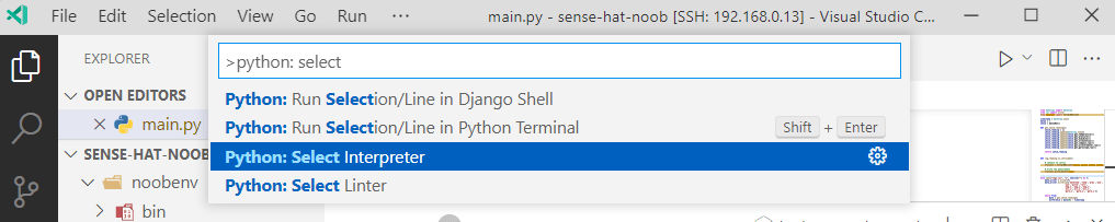
There is a library for working with InfluxDB hosted on PyPi. We need to download and install the packages locally. Remembering to use our Python virtual environment. Though this time we are going to give the VS Code Python environments integration the spotlight. Invoke the Command Palette Ctrl + Shift + P. Start typing and select the option for “Python: Select Interpreter“.
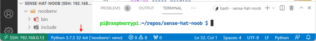
Look what VS Code recommends…
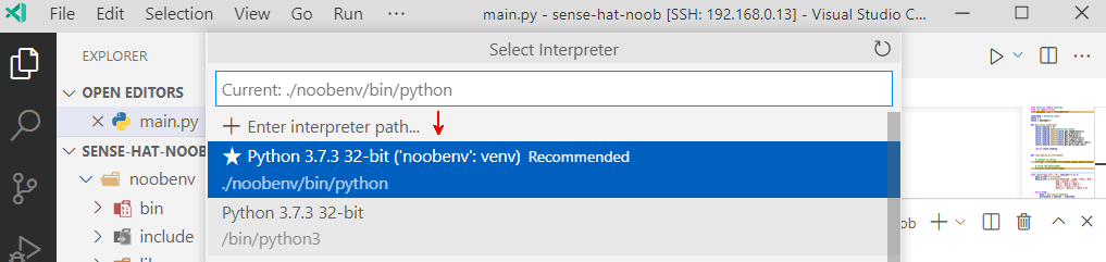
Our virtual environment. It’s so smart. I think it reads my blog drafts 🤣. After we chose the interpreter, VS Code switches context to our virtual environment context. It even reminds us in the status bar at the bottom of the window. So thoughtful!
🚧 Slight detour 🚧
Slight digression from our regular blog flow...
Now, if you are briskly following along and haven’t switched to the venv in the terminal, then you will probably run into an error like this. Which might lead you on a wild goose chase across fields of learnings and wonder.
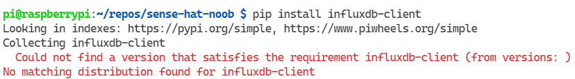
Naturally, we go looking to see if we find any packages for influxdb-client:
pip search influxdb-clientWhich the PyPI XMLRPC API politely, in a crimson message, lets us know things are not as peachy as we hoped:
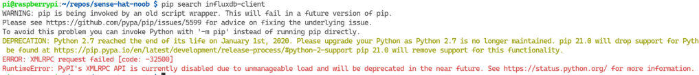
Fault: <Fault -32500: “RuntimeError: PyPI’s XMLRPC API is currently disabled due to unmanageable load and will be deprecated in the near future. See https://status.python.org/ for more information.”>
After updating the pip version in the venv, we check on the status which the error message suggested. After a very interesting read, a smidge of despair, hope emerges… I said to myself, “Self, why does that terminal not have the venv prefix?“. That’s when I realised the true source of the problem. Me. I forgot to activate the venv 😅.
For the terminal we still need to activate the virtual environment. To do this on the Pi we can run:
source <yourvenv>/bin/activate
Behold!!! It lives!!
When we do that, the terminal actually changes a little, giving us a visual cue that we are in a Python virtual environment. Now to get supporting packages installed so that we can write Python code for InfluxDB. Taking a look at the InfluxDB Client Python GitHub Repo or the influxdb-client PyPI project.
pip install influxdb-client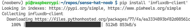
Sometimes Python can’t catch the programmer being the error.
~ me
🚧 Slight detour ends 🚧
The packages are installed. The logging can begin. To get started we need to import the influxdb_client into our project.
from sense_hat import SenseHat
from datetime import datetime
from influxdb_client import InfluxDBClient, Point
Yet again, we find a pebble in our shoe… While trying to import the sense_hat library modules in the REPL an error presented itself which seemed related to the way the numpy library was installed.
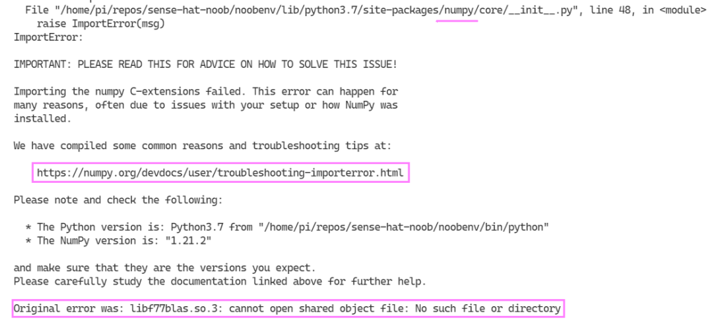
The error message helps a ton! Jumping over to the common reasons and troubleshooting tips helps with options to solve the issue on a Raspberry Pi, if we use our original error “libf77blas.so.3: cannot open shared object file: No such file or directory“. I opted for the first option to install the package with apt-get:
sudo apt-get install libatlas-base-devThen tried to enter the python REPL again (just typing “python” while in the terminal) and importing the SenseHat module.

I am beginning to feel like a module hunter 🏹. I tracked down a RaspberryPi thread which led me to a comment on a GitHub issue for the RTIMU module error. To be clear, this doesn’t seem to be an issue when I am running in the global Python scope. Only an issue in the virtual environment. The folks were kind enough to provide a way to install this with a pip command. Here we go:
pip install rtimulib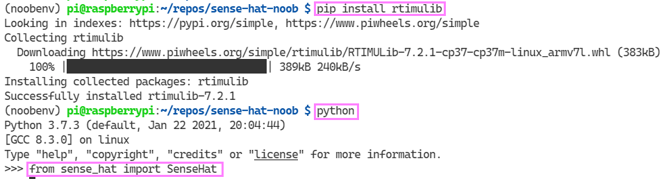
Yes! It works!
I tried initially to write a Python function that would write to and query the database. It wasn’t long before I ran into an error trying to connect to the database using the Python function.

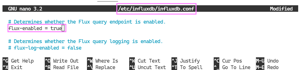
For v1.8 it’s disabled and we need to enable it. To edit the file we can use nano a Linux Command Line text editor.
[http]

  # ...

  flux-enabled = true

  # ...
sudo nano /etc/influxdb/influxdb.confWhich opens the file in nano for us to edit.
The settings are changed. To bring them into effect we need to restart the service.
sudo systemctl restart influxdb.service
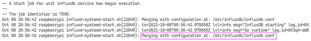
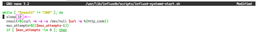
No much to go on. I found what seems to be a potential workaround. There is a comment further down in this thread on InfluxDB not starting that talks about adjusting a sleep setting for a start up file. Worth a try. Using nano again, we open the file and make the change.

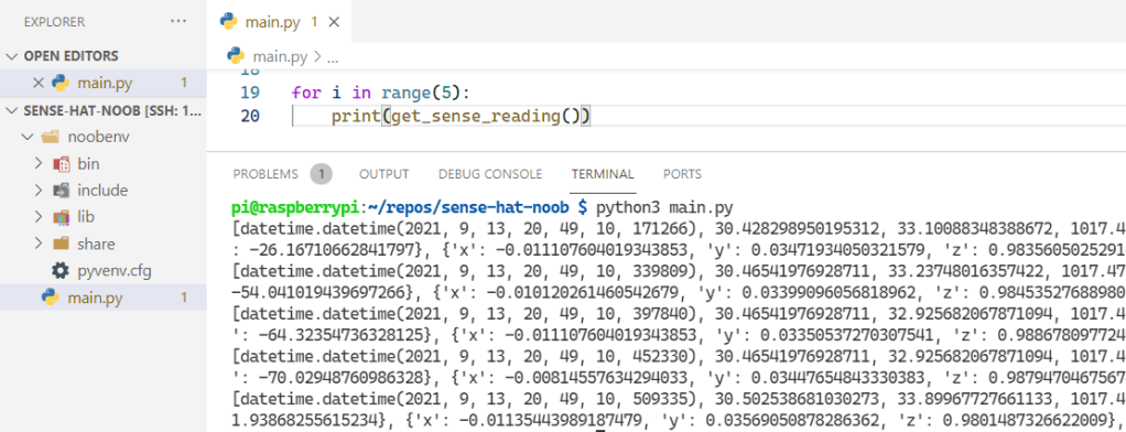
Time to write the code that will log records to our database. The idea is simple. Run a loop. Every few seconds get a Sense HAT reading. Log the reading to our InfluxDB. Stop the loop when we interrupt the program.
from sense_hat import SenseHat
from datetime import datetime
from influxdb_client import InfluxDBClient, Point

timestamp = datetime.now()
delay = 15
sense = SenseHat()
host = "localhost"
port = 8086
username = "grafanabaggins"
password = "<NotMyPrecious>"
database = 'shire'
retention_policy = 'autogen'
bucket = f'{database}/{retention_policy}'

def get_sense_reading():
    sense_reading = []
    sense_reading.append(datetime.now())
    sense_reading.append(sense.get_temperature())
    sense_reading.append(sense.get_pressure())
    sense_reading.append(sense.get_humidity())
    return sense_reading

# This method will log a sense hat reading into influxdb
def log_reading_to_influxdb(data, timestamp):
    point = ([Point("reading").tag("temperature", data[1]).field("device", "raspberrypi").time(timestamp), Point("reading").tag("pressure", data[2]).field("device", "raspberrypi").time(timestamp), Point("reading").tag("humidity", data[3]).field("device", "raspberrypi").time(timestamp)])
    client = InfluxDBClient(url="http://localhost:8086", token=f"{username}:{password}", org="-")
    write_client = client.write_api()
    write_client.write(bucket=bucket, record=point)

# Run and get a reading Forrest
def run_forrest(timestamp):
    try:
        data = get_sense_reading()
        log_reading_to_influxdb(data, timestamp)
        while True:
            data = get_sense_reading()
            difference = data[0] - timestamp
            if difference.seconds > delay:
                log_reading_to_influxdb(data, timestamp)
                sense.show_message("OK")
                timestamp = datetime.now()
    except KeyboardInterrupt:
        print("Stopped by keyboard interrupt [CTRL+C].")
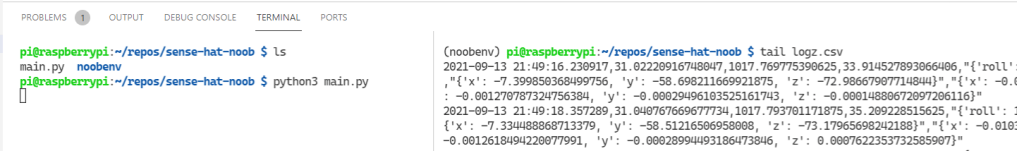
I struggled for a while trying to figure out the bucket/token variable to what I was able to do in the 1.8.9 CLI easily. I revisited the Python client library and noticed a specific callout for v1.8 API compatibility which has an example that helped me define the token. It wasn’t long before we got the script running and data was being logged to the database.
We’re getting there!
To the Shire
Before we get started on logging data to the database we need to understand some key concepts in InfluxDB. It won’t be the last time I visit that page, these concepts are foreign to me. I learnt to use InfluxQL which is a SQL language to work with the data. There are some differences between Flux and InfluxQL that you might want to keep in mind. I had a tricky time figuring out how to execute Flux queries initially after I wasn’t getting any data back from my Flux commands in a Python function, but saw that you could invoke a REPL to test queries with). To keep things simple though, I opted for InfluxQL. We can launch the Influx CLI from the terminal and query our data.
influx

SHOW DATABASES

USE <database>

SELECT * FROM <table>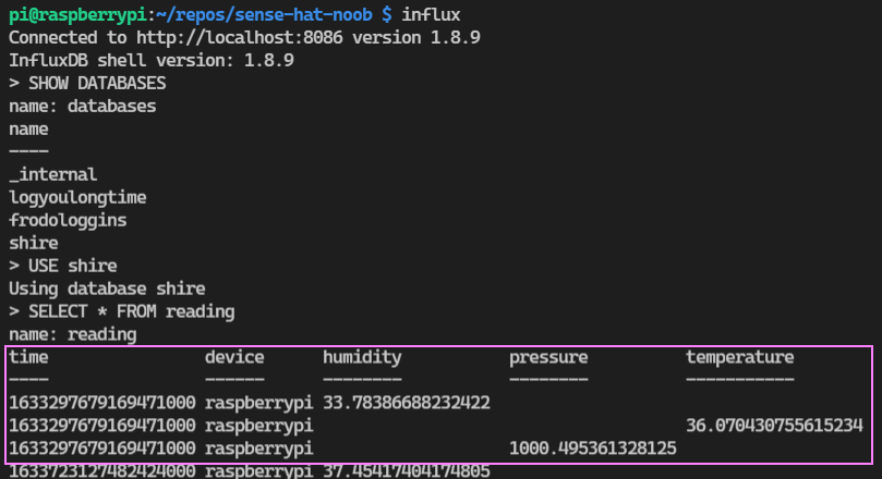
Let’s see if we can build a dashboard to visualise the data we are logging. We can connect to our Grafana server again. Head to the home page. There is a “Explore” menu item that is a quick way for us to query our data and experiment. Once the window opens up we select our data source connection from the drop down box and begin building a query with a wonderfully simple interface.
It’s at this point we realise that our logging design might not be correct. What I was expecting was that I could use the columns in the SELECT and WHERE clauses. Apparently not. I initially thought that design would work better because I understood that tags were indexed, not fields, so querying the tags would be faster. Good in theory, but I couldn’t reference the tag in the SELECT and WHERE clauses. My initial mental model needed tweaking. A change to the logging function to log to a single point, not three, with multiple fields.
So this:
point = ([Point("reading").tag("temperature", data[1]).field("device", "raspberrypi").time(timestamp), Point("reading").tag("pressure", data[2]).field("device", "raspberrypi").time(timestamp), Point("reading").tag("humidity", data[3]).field("device", "raspberrypi").time(timestamp)])Changed to this:
point = ([Point("reading").tag("device","raspberrypi").field("temperature", data[1]).field("pressure", data[2]).field("humidity", data[3]).time(timestamp)])
Minor InfluxDB management needed in future to clean up the database. For now though, we have our ‘frodologgins‘ database which is empty. I ran the logging function against the new database and…
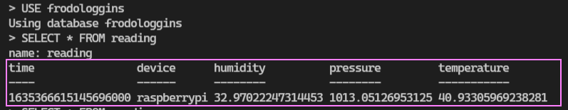
It works as expected! A quick updated to the Grafana connection settings to switch to the new database. With the updates in place we now get the expected results in the drop down. We can see the fields we want to display and chart.
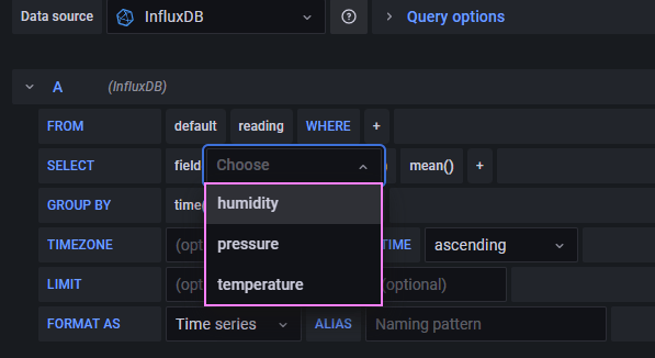
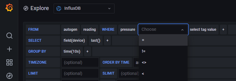
We can try reconcile the point, tags, and field in the Python code to how we are querying it with InfluxQL. Slowly sharpening our mental model and skills. The query reads as follows:
- From our database
- Query our readings for the default/autogen retention policy
- Where the device tag value is raspberrypi
- Return the last temperature field reading
- Group by ten second intervals

One thing I wasn’t quite sure of is the way that the time range worked in Grafana with the data logged in the database. The query looked correct but no data was returned. I was looking at a window from now-1d to now initially. It seemed logical to me, “find me all the data points from yesterday to now“. The Inspector in Grafana helps get the query and then we can use that to run the query in the Influx CLI to test the queries.
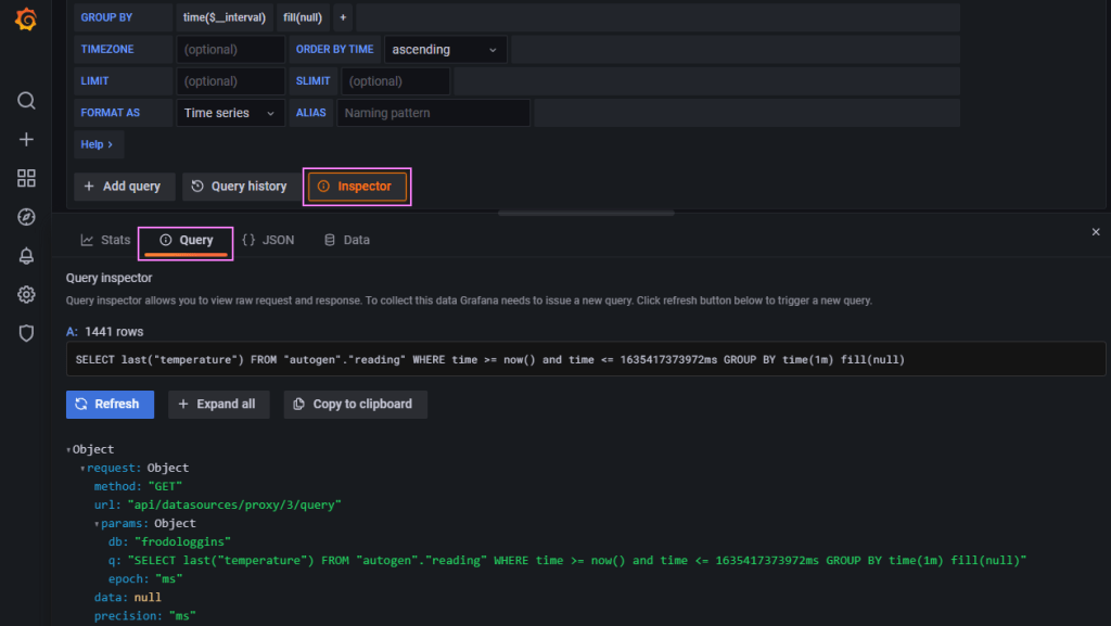
I eventually adjusted that to now to now+1d which in my mind is “back to the future” 🔮🚗, but it worked. I think this comes down to how the dates are stored (i.e. timezone offsets) and the functions evaluation. I’ll dig into that later, for now this works, we have data showing on a graph.

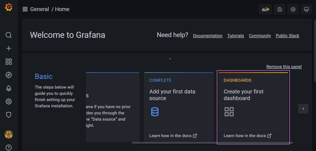
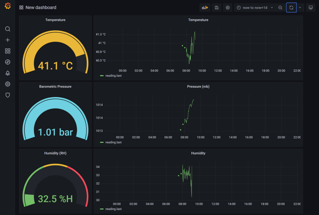
Let’s take the learnings and apply it to building the dashboard. Head to the home page. There is a “Dashboards” tile we can use to build our first dashboard.
It opens up a new editing window. I chose an empty panel. From there we can edit the panel in a similar way to what we did with the Explore window. In the upper right corner we can choose the type of chart.
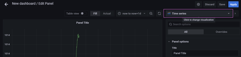
There are a bunch of options from changing the charts, adjusting threshold values for the gauges, applying units of measure, and so much more. For our case that’s “Time series“.
That’s it! Use the same approach to build out the other charts. I added “Gauge” visuals as well with the corresponding query.
Learnings 🏫
We made it! It took a while but we did it. Failure is a pretty good teacher. I failed a bunch and learnt a more. That’s not wasted time. It’s worth just getting hands on and trying different things out to build the mental model and skills. I have a long way to go to really understand Python, InfluxDB, Grafana, and Linux but I’ve made progress and learnt new things which is a blessing.
Until next time.
🐜